Building Blocks
PRISM was created to conduct "full-up" analyses of propulsion systems, however, by its nature it also contains the building blocks to conduct smaller, more focused tasks such as those described below.
Look up Fluid Properties
The following script.
#from prism.props.refprop7.n_dll_fluid import n_fluid
from engcoolprop.ec_fluid import EC_Fluid

h = EC_Fluid("N2")

h.setPD( P=50.0, D=0.1)
h.printTPD()
h.setTP(T=400.0, P=500.0)
h.printTPD()
h.constS_newP(P=1000.0)
h.printTPD()
Gives Output:
N2 T=1303.3 P=  50.0 D=0.1000 E=235.32 H=327.91 S=1.771 Q=4.74
N2 T= 400.0 P= 500.0 D=3.4128 E= 66.10 H= 93.23 S=1.299 Q=999.00
N2 T= 491.3 P=1000.0 D=5.4081 E= 80.12 H=114.36 S=1.299 Q=999.00
Look up CEA Isp
Bipropellant
The following script.
from prism.isp.cea.CEA_Isp import CEA_Isp

Pc=200.0
MR=1.0
eps=10.0

print 'at Pc=%g psia, MR=%g, Area Ratio=%g'%(Pc,MR,eps)

ispObj = CEA_Isp(propName='', oxName='LOX', fuelName="CH4")
IspODE, Cstar, Tcomb = ispObj.get_IvacCstrTc(Pc=Pc, MR=MR, eps=eps )

print 'for propellant =',ispObj.desc
print 'IspODE=%g sec, Cstar=%g ft/sec, Tcomb=%g degR'%(IspODE, Cstar, Tcomb)
Gives Output:
at Pc=200 psia, MR=1, Area Ratio=10
reading cea isp data files for LOX / CH4
for propellant = LOX / CH4
IspODE=246.205 sec, Cstar=4427.22 ft/sec, Tcomb=2076.43 degR
Monopropellant
The following script.
from prism.isp.cea.CEA_Isp import CEA_Isp

Pc=200.0
eps=10.0

print 'at Pc=%g psia, Area Ratio=%g'%(Pc,eps)

ispObj = CEA_Isp(propName="HAN315")
IspODE, Cstar, Tcomb = ispObj.get_IvacCstrTc(Pc=Pc, eps=eps )

print 'for propellant =',ispObj.desc
print 'IspODE=%g sec, Cstar=%g ft/sec, Tcomb=%g degR'%(IspODE, Cstar, Tcomb)
Gives Output:
Config File: C:\Users\Charlie\PRISM.cfg
Refprop dll_path = C:/RefProp8/
at Pc=200 psia, Area Ratio=10
reading cea isp data files for  HAN315
for propellant =  HAN315
IspODE=241.309 sec, Cstar=4499.55 ft/sec, Tcomb=3731.46 degR
Solid Propellant
The following script.
from prism.isp.cea.CEA_Isp import CEA_Isp

Pc=200.0
eps=10.0

print 'at Pc=%g psia, Area Ratio=%g'%(Pc,eps)

ispObj = CEA_Isp(propName="ARC448")
IspODE, Cstar, Tcomb = ispObj.get_IvacCstrTc(Pc=Pc, eps=eps )

print 'for propellant =',ispObj.desc
print 'IspODE=%g sec, Cstar=%g ft/sec, Tcomb=%g degR'%(IspODE, Cstar, Tcomb)
Gives Output:
Config File: C:\Users\Charlie\PRISM.cfg
Refprop dll_path = C:/RefProp8/
at Pc=200 psia, Area Ratio=10
reading cea isp data files for  ARC448
for propellant =  ARC448
IspODE=228.243 sec, Cstar=4290.93 ft/sec, Tcomb=3455.97 degR
Calculate TDK Isp
The following script.
from prism.isp.tdk import TDKwrap

tdk = TDKwrap.TDK( oxName='O2', fuelName='CH4',raoNozzle=0, varGammaRao=0,
    fracFuelL=None, fracOxL=None,
    MR=3.0, eps=150.0, Rthrt=1.0,
    Pc=250.0,  THETAB=25.0,
    RWTU = 1.0, RWTD = 1.0, calcBL=1,  IWALL=4, THETAI=30.0, ScarfAng=0.0,
    SkewParabTheta=None, SkewParabExitAng=None,
    pcentBell=74.0, Pamb=0.0, findOptParab=0, saveFile='ame_nom', useDBruns=1,
    inpNozContour=None)

print    'tdk.Isp ', tdk.Isp
print    'tdk.Cstar',tdk.Cstar
print    'tdk.etaKin1D',tdk.etaKin1D
print    'tdk.etaKin2D',tdk.etaKin2D

print 'Pexit=',tdk.Pexit
print
print 'IspTDK_wBL=',tdk.IspTDK_wBL
print 'IspODE=',tdk.IspODE
Gives Output:
tdk.Isp  369.1169
tdk.Cstar 6127.79
tdk.etaKin1D 0.973964333441
tdk.etaKin2D 0.966432474834
Pexit= 0.1008

IspTDK_wBL= 364.932178
IspODE= 381.9376
Matplotlib Graph of CEA Output
A matplotlib chart of LOX/LH2 CEA data can be created as shown below.
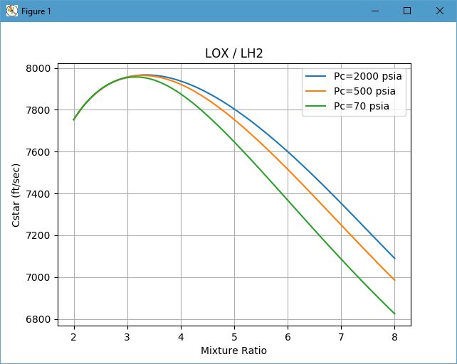
The above chart was created by the following script.
from prism.isp.cea.CEA_Isp import CEA_Isp
from pylab import *

Pc = 500.0
pcL = [ 2000., 500., 70.]

ispObj = CEA_Isp(propName='', oxName='LOX', fuelName="LH2")

for Pc in pcL:
    cstarArr = []
    MR = 2.0
    mrArr = []
    while MR < 8.0:
        cstarArr.append( ispObj.get_Cstar( Pc=Pc, MR=MR) )
        mrArr.append(MR)
        MR += 0.05
    plot(mrArr, cstarArr, label='Pc=%g psia'%Pc)

legend(loc='best')
grid(True)
title( ispObj.desc )
xlabel( 'Mixture Ratio' )
ylabel( 'Cstar (ft/sec)' )
savefig('cea_cstar_plot.png', dpi=120)

show()
Excel Graph of CEA Output
An Excel chart of LOX/LH2 CEA data can be created as shown below.
Cstar
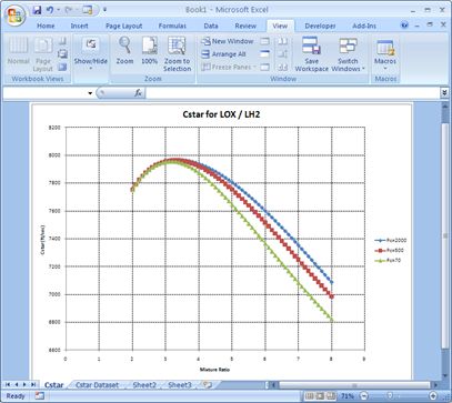
The above chart was created by the following script.
from prism.utils import xlChart
from numpy import arange
from prism.isp.cea.CEA_Isp import CEA_Isp

pcL = [ 2000., 500., 70.]

topRow = ['MR']
for Pc in pcL:
    topRow.append( 'Pc=%g'%Pc )

rs = [topRow]

ispObj = CEA_Isp(propName='',
    oxName='LOX', fuelName="LH2")
mrL = arange(2.0,8.1,0.1)

for MR in mrL:
    row = [MR]
    for Pc in pcL:
        row.append( ispObj.get_Cstar( Pc=Pc, MR=MR) )
    rs.append(row)

xl = xlChart.xlChart()
xl.makeChart(rs, title="Cstar for "+ispObj.desc, nCurves = len(pcL),
             chartName="Cstar",
             sheetName="Cstar Dataset",
             yLabel="Cstar (ft/sec)", xLabel="Mixture Ratio")
Isp
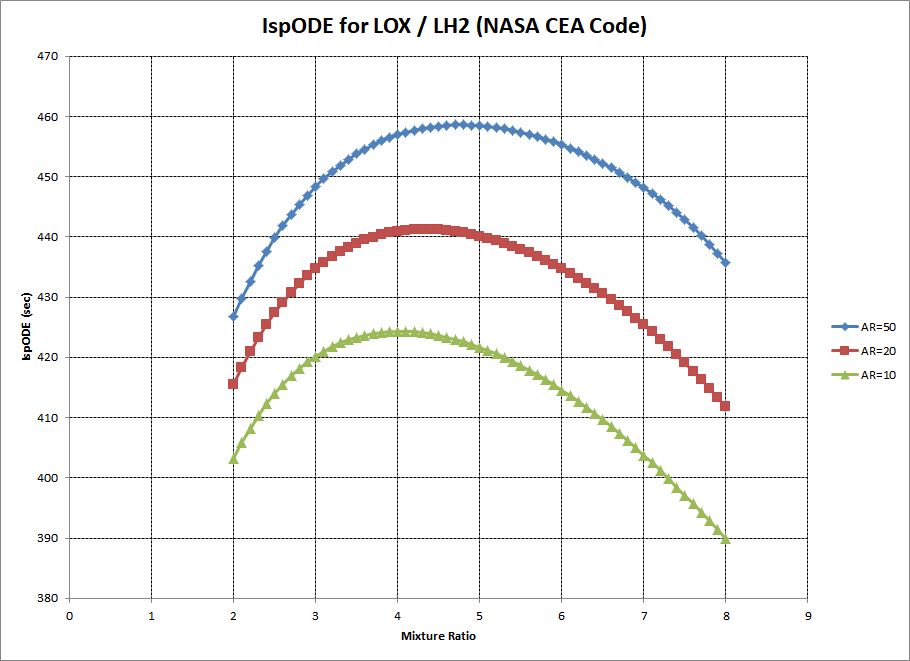
The above chart was created by the following script.
from prism.utils import xlChart
from numpy import arange
from prism.isp.cea.CEA_Isp import CEA_Isp

Pc = 500.0
epsL = [ 50., 20., 10.]

topRow = ['MR']
for eps in epsL:
    topRow.append( 'AR=%g'%eps )

rs = [topRow]

ispObj = CEA_Isp(propName='', oxName='LOX', fuelName="LH2")
mrL = arange(2.0,8.1,0.1)

for MR in mrL:
    row = [MR]
    for eps in epsL:
        IspODE, Cstar, Tcomb = ispObj.get_IvacCstrTc(Pc=Pc, MR=MR, eps=eps )
        row.append( IspODE )
    rs.append(row)

xl = xlChart.xlChart()
xl.makeChart(rs, title="IspODE for "+ispObj.desc+" (NASA CEA Code)", nCurves=len(epsL),
             chartName="IspODE",
             sheetName="IspODE Dataset",
             yLabel="IspODE (sec)", xLabel="Mixture Ratio")
TDK Delivered Isp
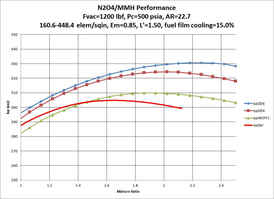
The above chart was created by the following script.
from prism import *
from prism.utils import xlChart

pcentFFC=15.0
etaPulse=1.0
mrBarrier=0.15
FvacGoal = 1200.0
elemDens=None # if None use d/v
Em=0.85

pc=500.0
eps=22.7
oxName= 'N2O4'
fuelName='MMH'

Tox=500.0    # Tox=None if using reference point
Tfuel=500.0  # Tfuel=None if using reference point

props = oxName + '/' + fuelName
mrLow=0.5
mrHigh=2.5
Nsteps = 25

LoverDt=0.1
LchamMin=1.5

rs = [ ['MRcore','IspODE','IspODK','IspWOFFC','IspDel','MRengine','Tcomb','CstarWOFFC','AreaRatio','Pc',
        'etaKin', 'etaDiv', 'etaBL', 'etaVap', 'etaMix', 'etaEm', 'etaFFC', 'etaPulse'] ]

delMR = (mrHigh-mrLow)/Nsteps

LprimeMin = 99999.0
LprimeMax = 0.0
elemDensMin = 99999.0
elemDensMax = 0.0

for i in range(Nsteps+1):
    mr = mrLow + i * delMR

    Engine = Engine_FFC(name="Est Engine",
                    oxName=oxName, fuelName=fuelName, etaERE=0.98,
                    Pc=pc, Fvac=FvacGoal, eps=eps, mr=mr, CR=2.5, LoverDt=LoverDt,  LchamMin=LchamMin,
                    pcentBell=80.0)

    if Engine.Lcham > LprimeMax: LprimeMax = Engine.Lcham
    if Engine.Lcham < LprimeMin: LprimeMin = Engine.Lcham

    LP = Lperf( engine = Engine ,Tox=Tox, Tfuel=Tfuel, elemDens=elemDens,
        pcentFFC=pcentFFC, mrBarrier=mrBarrier, etaPulse=etaPulse, Em=Em)

    if LP.elemDensCalc > elemDensMax: elemDensMax = LP.elemDensCalc
    if LP.elemDensCalc < elemDensMin: elemDensMin = LP.elemDensCalc

    IspWOFFC = LP.IspDel / LP.etaFFC
    rs.append( [mr, LP.IspODE, LP.IspODK, IspWOFFC,   LP.IspDel,LP.mrEngine,
        LP.TcombODE, LP.CstarDel, eps, pc,
        LP.etaKin, LP.etaDiv, LP.etaBL, LP.etaVap, LP.etaMix, LP.etaEm, LP.etaFFC, LP.etaPulse] )


print Engine.getSummary()
print LP.getSummary()

xl = xlChart.xlChart()

xl.xlApp.DisplayAlerts = 0  # Allow Quick Close without Save Message
#xl.makeDataSheet( _resultsRS, sheetName="Tank Fill")

if '%.2f'%LprimeMin=='%.2f'%LprimeMax:
    LprimeStr = "%.2f"%LprimeMin
else:
    LprimeStr = "%.2f-%.2f"%(LprimeMin,LprimeMax)


if '%.1f'%elemDensMin=='%.1f'%elemDensMax:
    elemDensStr = '%.1f'%elemDensMin
else:
    elemDensStr = '%.1f-%.1f'%(elemDensMin,elemDensMax)

if elemDens:
    myTitle = "%s Performance\nFvac=%.0f lbf, Pc=%.0f psia, AR=%.1f\n%.2f elem/sqin, Em=%.2f, L'=%s, fuel film cooling=%.1f%%"%\
        (props, FvacGoal, pc, eps, elemDens, Em, LprimeStr, pcentFFC)
else:
    myTitle = "%s Performance\nFvac=%.0f lbf, Pc=%.0f psia, AR=%.1f\n%s elem/sqin, Em=%.2f, L'=%s, fuel film cooling=%.1f%%"%\
        (props, FvacGoal, pc, eps, elemDensStr,  Em, LprimeStr, pcentFFC)

xl.makeChart(rs,
            title=myTitle,nCurves = 4,
            chartName="Performance",
            sheetName="FillData",yLabel="Isp (sec)", xLabel="Mixture Ratio")

xl.changeSeriesXValuesColumn( NColumn=6, NSeries=4)
#xl.putSeriesOnSecondary(2, y2Label="Temperature (degR)")
#xl.makeNewChartOfPlottedColumns(cols=(7,), ZeroBased=0, chartName='Quality')
#xl.changePlotTitle( 'Quality of %s'%tf.gasData.name )
#xl.labelPrimaryYAxis( 'Quality of %s (fraction gas)'%tf.gasData.name )
xl.labelXAxis( 'Mixture Ratio' )
xl.setXrange( 1.0, 2.5)
xl.setYrange( 250.0, 350.0)


xl.setLineThickness( NSeries=4, thickness=5)
xl.setSeriesColor( NSeries=4, red=255, green=0, blue=0)
xl.turnMarkerOnOff( NSeries=4, showPoints=0)
Calculate Friction Factor
The Colebrook equation is the most standard approach to calculating friction factor.
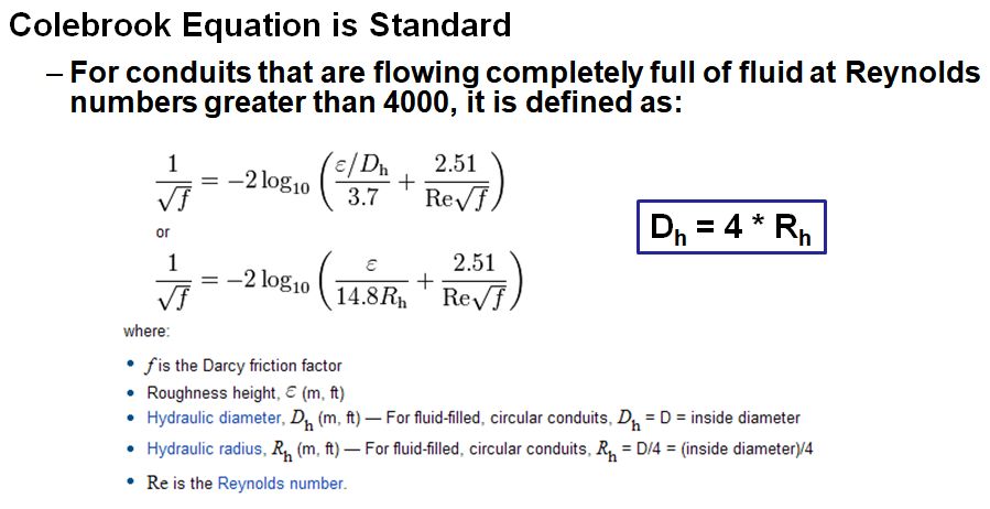
Because of Colebrook's iterative nature, however, other non-iterative equations are sometimes used:
Haaland Equation is Non-iterative
ffHaaland = (1.0/ (-1.8*log10((eod/3.7)**1.11 + 6.9/ReNum)) )**2

Buzzelli  Equation is Non-iterative
From the "Fluid Power" article for single pass evaluation of colebrook
by Dennis Buzzelli June 19, 2008

Transition from Laminar to Turbulent is at Reynolds Numbers from about 2300 to 4000
The following script calculates all three of these approaches.
from prism.utils.colebrook import colebrook_ffact, buzzelli_ffact
from math import log10

ReNum = 2.0E5
diam = 0.2
rough = 0.0001 # in
eod = rough / diam

ffColebrook = colebrook_ffact(rough,diam,ReNum)
ffBuzzelli = buzzelli_ffact(eod, ReNum)
ffHaaland = (1.0/ (-1.8*log10((eod/3.7)**1.11 + 6.9/ReNum)) )**2

print 'Colebrook:','%g'%ffColebrook
print 'Buzzelli :','%g'%ffBuzzelli, \
    '(%+.2f'%((ffBuzzelli-ffColebrook)*100.0/ffColebrook),'% Error)'
print 'Haaland  :','%g'%ffHaaland, \
    '(%+.2f'%((ffHaaland-ffColebrook)*100.0/ffColebrook),'% Error)'
Gives Output:
Colebrook: 0.0188198
Buzzelli : 0.0188215 (+0.01 % Error)
Haaland  : 0.0186371 (-0.97 % Error)
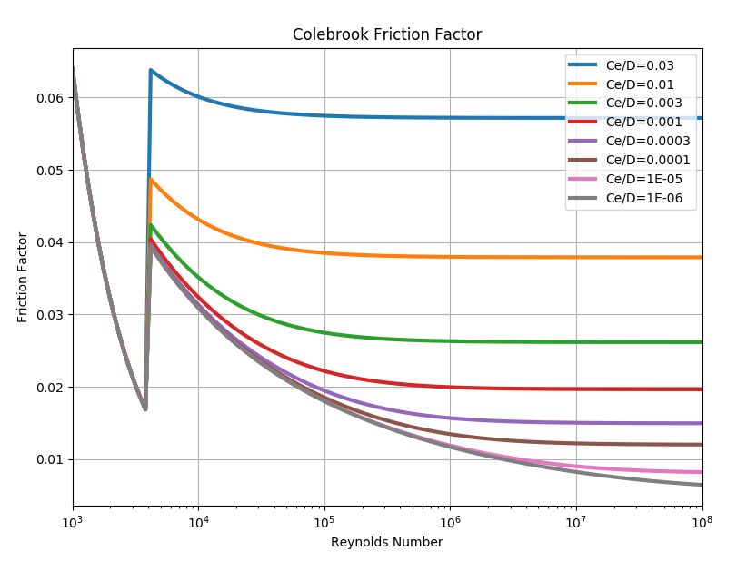
A graph of the Colebrook equation is created by the following script
from pylab import *
from prism.utils.colebrook import colebrook_ffact, buzzelli_ffact

e = 5.0e-6
diam = 1.0
eList = [.03, .01, .003, .001, .0003, .0001, .00001, .000001]

cycle = [1.0]
while cycle[-1]<10.0:
    cycle.append( cycle[-1] * 1.1 )
cycle = cycle[:-1]

ReList = [1.E3, 1.E4, 1.E5, 1.E6, 1.E7]

for e in eList:
    xRe = []
    yFF = []

    for ReBase in ReList:
        for cyVal in cycle:
            ReNum = ReBase * cyVal
            ff = colebrook_ffact(e,diam,ReNum)
            #print ReNum, ff
            xRe.append( ReNum )
            yFF.append( ff )

    #p.add( biggles.Curve(xRe, yFF, color="red") )

    semilogx(xRe,yFF,linewidth=3, label='Ce/D=%G'%e )

legend(loc='best')

grid(True)
title( "Colebrook Friction Factor" )
xlabel( "Reynolds Number" )
ylabel( "Friction Factor" )

ax = axes()
ax.set_xlim( (1.0E3, 1.0E8) )

show()
And gives the output:
Create a Nozzle Profile
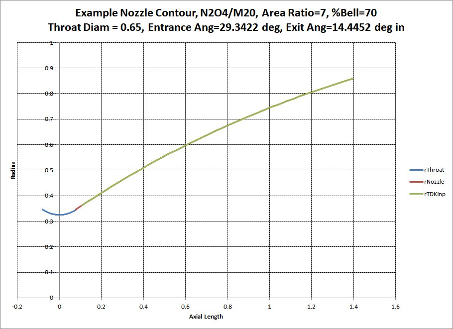
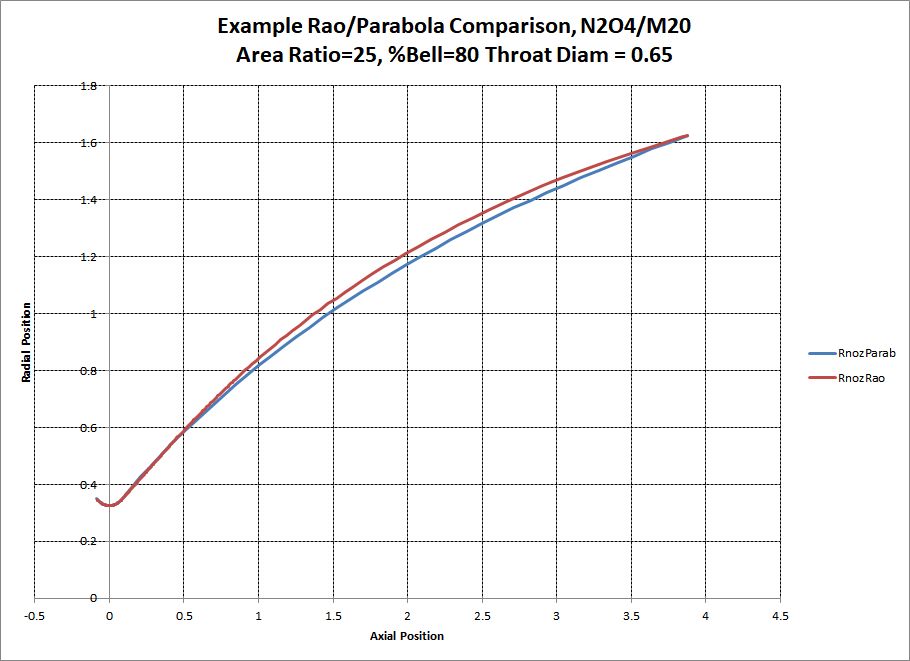
Nozzle contours are generally created as parabolic or Rao. Parabolic contours can be just as high performing as Rao, and may have better mechanical properties. (i.e. the entrance angle to the nozzle tends to be slightly smaller in parabolic than in Rao)
PRISM contains routines to create a parabolic contour and the TDK program has an option to create a Rao nozzle contour.
Parabolic
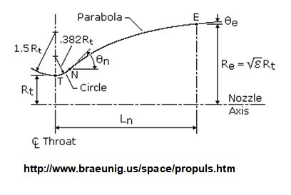
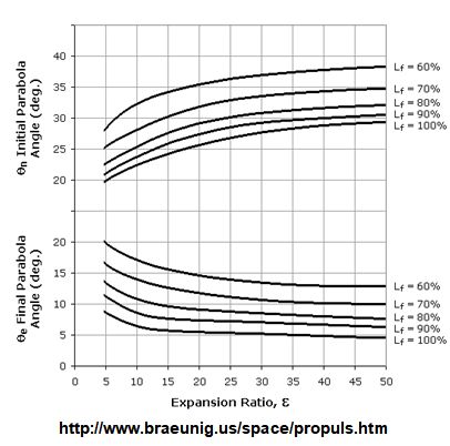
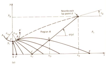
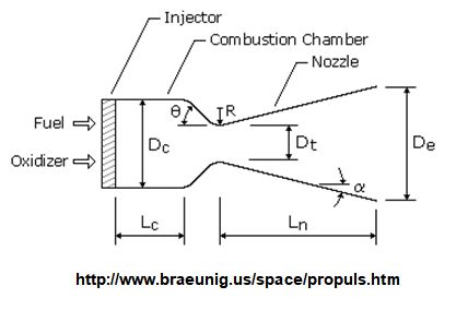
A parabolic contour is defined as shown below. There are general guidelines for choosing the entrance and exit angles of the nozzle as shown in the diagram.
The following script.
from prism.isp.tdk import raoContour, parabolic
from math import *
from prism.isp.cea.CEA_Isp import CEA_Isp


pc=400.0
pcentBell=70.0

eps=7.0
oxName= 'N2O4'
fuelName='M20'
mr = 1.0
Dthrt = 0.65
Rthrt = Dthrt/2.

ispObj = CEA_Isp(oxName=oxName, fuelName=fuelName)
IspODE, Cstar, Tcomb, mw, gam = ispObj.get_IvacCstrTc_ChmMwGam( Pc=pc, MR=mr, eps=eps)
print 'Using gamma =',gam

p = parabolic.Parabola(Rt=Rthrt, eps=eps, pcentBell=pcentBell, gam=gam,  Rd=0.5, showPlot=0)

myTitle = "Example Nozzle Contour, %s/%s, Area Ratio=%g, %%Bell=%g\nThroat Diam = %g, Entrance Ang=%g deg, Exit Ang=%g deg in"%\
    (oxName, fuelName, eps, pcentBell, Dthrt, p.theta, p.exitAng)
p.makeExcelPlots( title=myTitle, absUnits=1)
Creates an Excel spreadsheet with the following output:
Rao
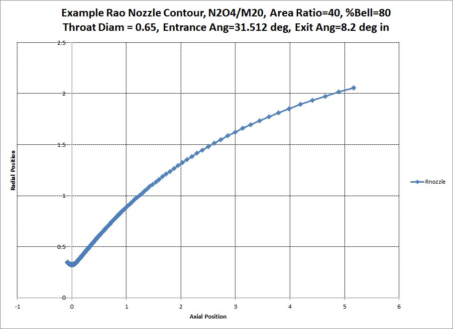
A Rao nozzle is designed by an optimized Method of Characteristics inside the TDK code.
The following script.
from prism.isp.tdk import raoContour, parabolic
from math import *
from prism.isp.cea.CEA_Isp import CEA_Isp
from prism.utils import xlChart

def sinDeg( ang ):
    return sin( ang*pi/180.0 )

def cosDeg( ang ):
    return cos( ang*pi/180.0 )

def isFloat(s):
    '''is the given string a float'''
    try: float(s)
    except ValueError: return 0
    else: return 1

pc=400.0
pcentBell=80.0

eps=40.0
oxName= 'N2O4'
fuelName='M20'
mr = 1.0
Dthrt = 0.65
Rthrt = Dthrt/2.

ispObj = CEA_Isp(oxName=oxName, fuelName=fuelName)
IspODE, Cstar, Tcomb, mw, gam = ispObj.get_IvacCstrTc_ChmMwGam( Pc=pc, MR=mr, eps=eps)
print 'Using gamma =',gam

rao = raoContour.RaoContour2( eps=eps, gam=gam, molWt=mw,
    Pc=pc, Tc=Tcomb, THETAB=25.0,
    RWTU = 2.0, RWTD = 0.5, RSTAR = 1.0,
    pcentBell=pcentBell, Lnoz=0.0, saveFile="testRao",
    useRao95=0, odeObj=None, useDBruns=0)

myTitle = "Example Rao Nozzle Contour, %s/%s, Area Ratio=%g, %%Bell=%g\nThroat Diam = %g, Entrance Ang=%g deg, Exit Ang=%g deg in"%\
    (oxName, fuelName, eps, pcentBell, Dthrt, rao.entranceAngle, rao.exitAngle )

rs = [ ['x','Rnozzle'] ]
# make the circular arc at the throat
ang = -rao.entranceAngle
while ang<=rao.entranceAngle:
    rs.append( [rao.RWTD*sinDeg(ang)*Rthrt, (1.0 + rao.RWTD*(1.-cosDeg(ang)))*Rthrt] )
    ang += 1.

rs.append( ['',''] ) # separate circular throat from detailed contour
# add the nozzle
for ZStar,RStar,MachNumber,Theta in rao.contourStar[3:]:
    if isFloat(RStar) and isFloat(ZStar):
        rs.append( [float(ZStar)*Rthrt, float(RStar)*Rthrt] )

xl = xlChart.xlChart()
xl.xlApp.DisplayAlerts = 0  # Allow Quick Close without Save Message

xl.makeChart(rs, title=myTitle ,nCurves = 1,
            chartName="Rao",sheetName="raoData",
            yLabel="Radial Position", xLabel="Axial Position")
Creates an Excel spreadsheet with the following output:
Compare Parabola Rao
To compare the two nozzle contours, run the following script.
from prism.isp.tdk import raoContour, parabolic
from math import *
from prism.isp.cea.CEA_Isp import CEA_Isp
from prism.utils import xlChart

def sinDeg( ang ):
    return sin( ang*pi/180.0 )

def cosDeg( ang ):
    return cos( ang*pi/180.0 )

def isFloat(s):
    '''is the given string a float'''
    try: float(s)
    except ValueError: return 0
    else: return 1

pc=400.0
pcentBell=80.0

eps=25.0
oxName= 'N2O4'
fuelName='M20'
mr = 1.0
Dthrt = 0.65
Rthrt = Dthrt/2.

ispObj = CEA_Isp(oxName=oxName, fuelName=fuelName)
IspODE, Cstar, Tcomb, mw, gam = ispObj.get_IvacCstrTc_ChmMwGam( Pc=pc, MR=mr, eps=eps)
print 'Using gamma =',gam

p = parabolic.Parabola(Rt=Rthrt, eps=eps, pcentBell=pcentBell, gam=gam,  Rd=0.5, showPlot=0)

rao = raoContour.RaoContour2( eps=eps, gam=gam, molWt=mw,
    Pc=pc, Tc=Tcomb, THETAB=25.0,
    RWTU = 2.0, RWTD = 0.5, RSTAR = 1.0,
    pcentBell=pcentBell, Lnoz=0.0, saveFile="",
    useRao95=0, odeObj=None, useDBruns=0)

myTitle = "Example Rao/Parabola Comparison, %s/%s\nArea Ratio=%g, %%Bell=%g Throat Diam = %g"%\
    (oxName, fuelName, eps, pcentBell, Dthrt)

rsP = [ ['x','RnozParab'] ]
# make the circular arc at the throat
ang = -p.theta
while ang<=p.theta:
    rsP.append( [p.Rd*sinDeg(ang)*Rthrt, (1.0 + p.Rd*(1.-cosDeg(ang)))*Rthrt] )
    ang += 1.

rsP.append( ['',''] ) # separate circular throat from parabola
# add the parabola
for i, xval in enumerate( p.zContour ):
    row = [xval * Rthrt,  p.rContour[i] * Rthrt]
    rsP.append(row)


rsR = [ ['x','RnozRao'] ]
# make the circular arc at the throat
ang = -rao.entranceAngle
while ang<=rao.entranceAngle:
    rsR.append( [rao.RWTD*sinDeg(ang)*Rthrt, (1.0 + rao.RWTD*(1.-cosDeg(ang)))*Rthrt] )
    ang += 1.

rsR.append( ['',''] ) # separate circular throat from detailed contour
# add the nozzle
for ZStar,RStar,MachNumber,Theta in rao.contourStar[3:]:
    if isFloat(RStar) and isFloat(ZStar):
        rsR.append( [float(ZStar)*Rthrt, float(RStar)*Rthrt] )

rs = xlChart.combineRS( rsP, rsR )

xl = xlChart.xlChart()
xl.xlApp.DisplayAlerts = 0  # Allow Quick Close without Save Message

xl.makeChart(rs, myTitle ,nCurves = 1,
            chartName="RaoParab",sheetName="raoParabData",
            yLabel="Radial Position", xLabel="Axial Position")

xl.addNewSeriesToCurrentSheetChart( xColumn=3, yColumn=4)
xl.turnMarkersOnOff( showPoints=0)
Creates an Excel spreadsheet that compares the two contours:
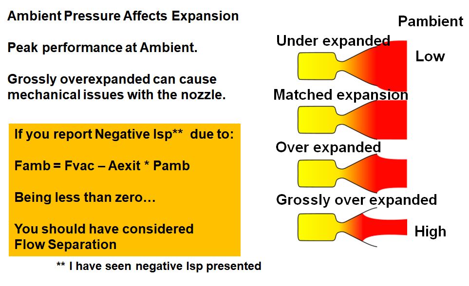
Nozzle Flow Separation
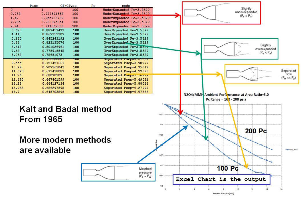
The following script runs nozzle separation calculations.
from prism.isp import separated_Cf
from prism.utils import xlChart
from prism.isp.cea.CEA_Isp import CEA_Isp

Fvac = 110.0
pc=108.0
eps=5.0
oxName= 'N2O4'
fuelName='MMH'
mr = 1.65
Nsteps = 20

ispObj = CEA_Isp(oxName=oxName, fuelName=fuelName)

IspODE, Cstar, Tcomb, mw, gam = ispObj.get_IvacCstrTc_ChmMwGam( Pc=pc, MR=mr, eps=eps)
print 'Using gamma =',gam

pcArr = [100.0, 150.0, 200.0]

rs = [ [ 'Pamb','Cf/Cfvac', 'Pc','mode'] ]
for pc in pcArr:
    for i in range( Nsteps+1):
        Pamb = 14.7 * i / Nsteps
        Cf, CfOverCfvac, mode = separated_Cf.ambientCf(gam=gam, epsTot=eps, Pc=pc, Pamb=Pamb)

        rs.append( [ Pamb, CfOverCfvac, pc, mode] )
    rs.append(['','','',''])

xl = xlChart.xlChart()
xl.xlApp.DisplayAlerts = 0  # Allow Quick Close without Save Message

myTitle = "%s/%s Ambient Performance at Area Ratio=%.1f\n"%(oxName, fuelName, eps) +\
    "Pc Range = %g - %g psia"%(min(pcArr), max(pcArr))
xl.makeChart(rs,
            title=myTitle,nCurves = 1,
            chartName="Performance",
            sheetName="FillData",yLabel="Cfamb/Cfvac", xLabel="Ambient Pressure (psia)")
xl.setYrange( 0.6, 1.0)
The script creates an Excel spreadsheet of nozzle separation calculations. A table of nozzle conditions is shown in the upper left corner of the image below. A graph of ambient pressure vs nozzle Cf ambient divided by Cf vacuum is shown in the bottom right corner of the image below:
Solve Nozzle Exit Diameter
The following script.
from prism import Goal
from prism import Engine_FFC

EngineDivert = Engine_FFC(name="Divert Engine",
    oxName='N2O4', fuelName='MMH', Number=4,
    cxw=1.0, Pc=200.0, Fvac=1000.0, eps=10.0, mr=1.65,
    CR=2.5, LoverDt=2.0, LchamMin=1.5, cxwValves=1.0,
    etaERE=0.97, calcEtaNoz=1, useFastCEALookup=1,isBell=1, pcentBell=80.,
    halfAngDeg=15.0, xlnOverLcham=0.9)


print 'Find Area Ratio that has Exit Diameter = 5.0 inches'
print
print 'Initial AR =',EngineDivert.eps,' Dexit =',EngineDivert.Dexit

def newDexit( e ):
    EngineDivert.eps = e
    EngineDivert.reCalc()
    return EngineDivert.Dexit

G = Goal(goalVal=5.0, minX=2.0, maxX=80.0,
    funcOfX=newDexit, tolerance=1.0E-5, maxLoops=40, failValue=80.0)
eps, ierror = G()
print
print 'Area Ratio =',eps,'for Dexit =',EngineDivert.Dexit

print EngineDivert.getSummary()
Gives Output:
Find Area Ratio that has Exit Diameter = 5.0 inches
Initial AR = 10.0  Dexit = 6.1915743957
Area Ratio = 6.30835836802 for Dexit = 5.00000001086

Bipropellant Engine: Divert Engine
             mass =       49.792 lbm
             type = inert
        Propellants : N2O4 / MMH
        NASA CEA Code for ODE performance
        Physical Weight Model
        Injector Material is SS
        Nozzle Material is Cb103
        Bell Nozzle with Percent Bell = 80
        Mass is for 4 engines total
     ==== INPUT ====
        Fvac            = 1000 lbf
        Pc              = 200.0 psia
        eps             = 6.30836
        %Bell           = 80.00 %
        mr              = 1.65
        CR              = 2.5
        xlnOverLcham    = 0.9
        LoverDt         = 2
        LchamMin        = 1.500 in
        cxwInj          = 1
        cxwValves       = 1
        cxw             = 1
        etaERE          = 0.97
     ==== OUTPUT ====
        Isp             = 276.997 sec
        Cstar           = 5547.8 ft/sec
        etaBL           = 0.991001
        etaDiv          = 0.983664
        etaKin          = 0.984052
        etaNoz          = 0.959266
        effIsp          = 0.930488
        IspODE          = 297.69 sec
        CstarODE        = 5719.4 ft/sec
        Tc              = 5544.0 degR
        PcFace          = 209.609 psia
        Pexit           = 4.44532 psia
        wdotTot         = 3.61015 lbm/sec
        wdotOx          = 2.24783 lbm/sec
        wdotFl          = 1.36232 lbm/sec
        rhoFl           = 0.0316 lbm/cuin
        rhoOx           = 0.0521 lbm/cuin
        volDotOx        = 43.1645 cuin/sec
        volDotFl        = 43.1597 cuin/sec
        DFlow           = 1.353 in
        At              = 3.11253 sqin
        Dt              = 1.991 in
        Dcham           = 3.148 in
        Dexit           = 5.000 in
        Lcham           = 3.981 in
        xlc             = 0.398 in
        xln             = 3.583 in
        Lnoz            = 4.492 in
        Lengine         = 11.621 in
        rhoInj          = 0.280 lbm/cuin
        rhoNoz          = 0.310 lbm/cuin
        thkCham         = 0.026 in
        thkNoz          = 0.021 in
        WtNoz           = 0.778 lbm
        WtChamber       = 0.262 lbm
        WtInj           = 3.954 lbm
        WtAcoustic      = 2.804 lbm
        WtValves(2)     = 4.292 lbm
        WtMisc          = 0.357 lbm
        wt/Engine       = 12.448 lbm
        F/W             = 80.334 lbf/lbm
Solenoid Valve: biprop valves
             mass =        4.292 lbm
             type = inert
        Based on Solenoid Valve Experience
        Mass is for 2 valves total
     ==== INPUT ====
        cuInchPerSec    = 43.1645 cuin/sec
        cxw             = 1.000
     ==== OUTPUT ====
        basemass        = 2.146 lbm
Size a Liquid Engine
The following script.
from prism import Engine_FFC

EngineDivert = Engine_FFC(name="Divert Engine",
    oxName='N2O4', fuelName='MMH', Number=4,
    cxw=1.0, Pc=200.0, Fvac=1000.0, eps=10.0, mr=1.65,
    CR=2.5, LoverDt=2.0, LchamMin=1.5, cxwValves=1.0,
    etaERE=0.97, calcEtaNoz=1, useFastCEALookup=1,isBell=1, pcentBell=80.,
    halfAngDeg=15.0, xlnOverLcham=0.9)

print EngineDivert.getSummary()
Gives Output:
Bipropellant Engine: Divert Engine
             mass =       49.186 lbm
             type = inert
        Propellants : N2O4 / MMH
        NASA CEA Code for ODE performance
        Physical Weight Model
        Injector Material is SS
        Nozzle Material is Cb103
        Bell Nozzle with Percent Bell = 80
        Mass is for 4 engines total
     ==== INPUT ====
        Fvac            = 1000 lbf
        Pc              = 200.0 psia
        eps             = 10
        %Bell           = 80.00 %
        mr              = 1.65
        CR              = 2.5
        xlnOverLcham    = 0.9
        LoverDt         = 2
        LchamMin        = 1.500 in
        cxwInj          = 1
        cxwValves       = 1
        cxw             = 1
        etaERE          = 0.97
     ==== OUTPUT ====
        Isp             = 286.35 sec
        Cstar           = 5547.8 ft/sec
        etaBL           = 0.988751
        etaDiv          = 0.987664
        etaKin          = 0.980909
        etaNoz          = 0.95791
        effIsp          = 0.929173
        IspODE          = 308.177 sec
        CstarODE        = 5719.4 ft/sec
        Tc              = 5544.0 degR
        PcFace          = 209.609 psia
        Pexit           = 2.34259 psia
        wdotTot         = 3.49224 lbm/sec
        wdotOx          = 2.17441 lbm/sec
        wdotFl          = 1.31782 lbm/sec
        rhoFl           = 0.0316 lbm/cuin
        rhoOx           = 0.0521 lbm/cuin
        volDotOx        = 41.7547 cuin/sec
        volDotFl        = 41.75 cuin/sec
        DFlow           = 1.331 in
        At              = 3.01087 sqin
        Dt              = 1.958 in
        Dcham           = 3.096 in
        Dexit           = 6.192 in
        Lcham           = 3.916 in
        xlc             = 0.392 in
        xln             = 3.524 in
        Lnoz            = 6.320 in
        Lengine         = 13.332 in
        rhoInj          = 0.280 lbm/cuin
        rhoNoz          = 0.310 lbm/cuin
        thkCham         = 0.025 in
        thkNoz          = 0.021 in
        WtNoz           = 0.958 lbm
        WtChamber       = 0.249 lbm
        WtInj           = 3.825 lbm
        WtAcoustic      = 2.699 lbm
        WtValves(2)     = 4.220 lbm
        WtMisc          = 0.346 lbm
        wt/Engine       = 12.296 lbm
        F/W             = 81.325 lbf/lbm
Solenoid Valve: biprop valves
             mass =        4.220 lbm
             type = inert
        Based on Solenoid Valve Experience
        Mass is for 2 valves total
     ==== INPUT ====
        cuInchPerSec    = 41.7547 cuin/sec
        cxw             = 1.000
     ==== OUTPUT ====
        basemass        = 2.110 lbm
To create an image of an engine like below.
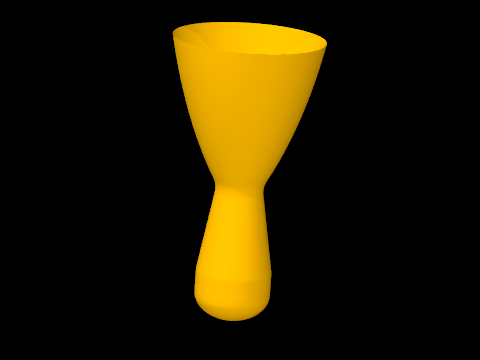
use the following script.
from prism.engines.Engine_FFC import Engine_FFC
from prism.pov.POV_Scene import POV_Scene

EngineDivert = Engine_FFC(name="Divert Engine",
    oxName='N2O4', fuelName='MMH', Number=4,
    cxw=1.0, Pc=200.0, Fvac=1000.0, eps=10.0, mr=1.65,
    CR=2.5, LoverDt=2.0, LchamMin=1.5, cxwValves=1.0,
    etaERE=0.97, calcEtaNoz=1, useFastCEALookup=1,isBell=1, pcentBell=80.,
    halfAngDeg=15.0, xlnOverLcham=0.9)

scene = POV_Scene(ambient=0.3)
scene.addItem( EngineDivert.getPOV_Item() )
scene.write(view="", ortho=1, clockX=-15., clockY=-15.)
scene.render()
Size a Tank
The following script.
from prism.tanks.Tank import Tank

oxekv = Tank(name="Divert Vehicle Propellant Tank",
    makeCompositeTank=1, kalmod=0,
    matlName="grEpox",   vfree=486.0,ell=1.767,rcyltd=1.445,
    ptank=1400.0,sf=1.5,cxw=1.5,
    ithcyl=1,kacqui=1,inpex=1,expefi=0.98,
    tblad=0.030,tbond=0.030,ttrspc=0.010,
    rhobnd=0.04,rhoacq=0.098,tliner=0.03,rholiner=0.098)

print oxekv.getSummary()
Gives Output:
Cylindrical/Spherical/Elliptical Tank: Divert Vehicle Propellant Tank
             mass =        3.763 lbm
             type = inert
        Composite Tank Algorithm
        Bladder Thickness is input at 0.030 in
        kalmod = 0
     ==== INPUT ====
        vfree           = 486 cuin
        vfreeTotal      = 486 cuin
        ell             = 1.767
        rcyltd          = 1.445
        ptank           = 1400 psia
        sf              = 1.5
        cxw             = 1.5
        ithcyl          = 1
        kacqui          = 1 transverse collapsing Alum. bladder
        inpex           = 1
        expefi          = 0.98
        tblad           = 0.030 in
        tbond           = 0.030 in
        ttrspc          = 0.010 in
        rhobnd          = 0.04 lbm/cuin
        rhoacq          = 0.098 lbm/cuin
        tliner          = 0.030 in
        rholiner        = 0.098 lbm/cuin
     ==== OUTPUT ====
        rinsid          = 3.535 in
        dinsid          = 7.069 in
        OR              = 3.618 in
        OD              = 7.237 in
        OH              = 14.385 in
        hinsid          = 14.215 in
        SAinsid         = 341.045 sqin
        cyl             = 10.215 in
        wacqui          = 0.987 lbm
        vacqui          = 9.87014 cuin
        dpacq           = 65.9344 psig
        pullag          = 1465.93 psia
        vresid          = 9.72 cuin
        vtank           = 505.59 cuin
        tming           = 0.008 in
        thkcyl          = 0.024 in
        thkend          = 0.025 in
        thkBladOut      = 0.030 in
        wliner          = 1.053 lbm
        wtank(+liner)   = 1.522 lbm
        rho             = 0.0637 lbm/cuin
        PmeopVoverW     = 188096 lbf-in/lbm
        Pburst(est.)    = 2100.0 psia
        PburstVoverW    = 282143 lbf-in/lbm
Size a Liquid Line
Input Diameter
The following script.
from prism import Line_Liq_inpD, Inc_liquid

Fl = Inc_liquid( symbol="N2H4",T=530.0,P=240.0, mass_lbm=10.0)

h = Line_Liq_inpD(name="Fuel Line",wdot=2.0, matlName="Ti", OD=0.5,
    liqObj=Fl, Number=10, Kfactors=5.0, pLine=400.0, thkWall=0.045)

print h.getSummary()
Gives Output:
Liquid Line: Fuel Line
             mass =        6.432 lbm
             type = inert
        fluid : N2H4
        Structural Material : Ti
        Mass is for 10 lines total
     ==== INPUT ====
        wdot            = 2 lbm/sec
        OD              = 0.500 in
        thkWall         = 0.045 in
        len_inches      = 50 in
        Kfactors        = 5 vel heads
        roughness       = 5e-06 in
        pLine           = 400 psia
        cxw             = 1.25
        # Lines         = 10
     ==== OUTPUT ====
        dpLine          = 58.05 psid
        dPperVelHead    = 8.15 psid
        velFPS          = 34.6998 ft/sec
        ReNum           = 1.214732E+05
        rinsid          = 0.205 in
        dinsid          = 0.410 in
        volLine         = 6.60127 cuin
        rho             = 0.16 lbm/cuin
        sy              = 119000 psi

        sf              = 65.3049
        tming           = 0.030 in
        fluid rho       = 0.0363801 lbm/cuin
        fluid visc      = 61.356 1.0E5 * lb/ft-sec
        wt/Line         = 0.643 lbm
Input Velocity
The following script.
from prism import Line_Liq, Inc_liquid

Fl = Inc_liquid( symbol="N2H4",T=530.0,P=240.0, mass_lbm=10.0)

h = Line_Liq(name="Fuel Line",wdot=2.0, matlName="Ti", velFPS=40.0,
    liqObj=Fl, Number=10, Kfactors=5.0, pLine=400.0)

print h.getSummary()
Gives Output:
Liquid Line: Fuel Line
             mass =        3.882 lbm
             type = inert
        fluid : N2H4
        Structural Material : Ti
        Allow Non-Standard wall thickness
        Mass is for 10 lines total
     ==== INPUT ====
        wdot            = 2 lbm/sec
        velFPS          = 40 ft/sec
        len_inches      = 50 in
        Kfactors        = 5 vel heads
        roughness       = 5e-06 in
        thkInp          = 0 in
        pLine           = 400 psia
        sf              = 4
        cxw             = 1.25
        # Lines         = 10
     ==== OUTPUT ====
        dpLine          = 78.53 psig
        ReNum           = 1.304208E+05
        thkLine         = 0.030 in
        rinsid          = 0.191 in
        dinsid          = 0.382 in
        doutside        = 0.442 in
        volLine         = 5.72658 cuin
        rho             = 0.16 lbm/cuin
        sy              = 119000 psi
        tming           = 0.030 in
        fluid rho       = 0.0363801 lbm/cuin
        fluid visc      = 61.356 1.0E5 * lb/ft-sec
        wt/Line         = 0.388 lbm
Size a Gas Line
Input Diameter
The following script.
from prism import Line_Gas

h = Line_Gas(name="Ox Line",wdot=1.0, matlName="Ti", thkWallInp=0.083,
    calcVelFromDiamInp=1, DiamInp=1.0,
    usePinlet=1, velFPS=20.0, PgasInlet=1000.0, TgasDegR=530.0,
    gasSymbol='O2', Number=10, Kfactors=2.0)

print h.getSummary()
Gives Output:
Gas Line: Ox Line
             mass =       23.911 lbm
             type = inert
        In: O2 T= 530.0 P=1000.0 D=5.8605 E= 76.25 H=107.85 S=1.255 Supercrit
        Out:O2 T= 529.9 P= 996.6 D=5.8410 E= 76.25 H=107.85 S=1.256 Supercrit
        fluid : O2
        Structural Material : Ti
        Allow Non-Standard wall thickness
        Using Pinlet to design line
        Line Diameter is an Input (vel is output)
        Mass is for 10 lines total
     ==== INPUT ====
        wdot            = 1 lbm/sec
        DiamInp         = 1.000 in
        thkWallInp      = 0.083 in
        len_inches      = 50 in
        Kfactors        = 2 vel heads
        roughness       = 5e-06 in
        PgasInlet       = 1000.0 psia
        sf              = 4
        cxw             = 1.25
        # Lines         = 10
     ==== OUTPUT ====
        PgasOutlet      = 996.6 psia
        velFPS          = 45.139 ft/sec
        velHead         = 1.289 psi
        dpLine          = 3.45 psig
        dp due to Line  = 0.89 psig
        dp due to Ks    = 2.56 psig
        dp/Pinlet       = 0.00344998
        ReNum           = 1.243308E+06
        fricfact        = 0.0116279
        thkLine         = 0.083 in
        rinsid          = 0.417 in
        dinsid          = 0.834 in
        volLine         = 27.3144 cuin
        rho             = 0.16 lbm/cuin
        sy              = 119000 psi
        tming           = 0.035 in
        fluid dens      = 5.86053 lbm/cuft
        fluid visc      = 1.47634e-05 lb/ft-sec
        fluid sonicV    = 1085.38 ft/sec
        fluid Mach      = 0.0415883
        wt/Line         = 2.391 lbm
Input Velocity
The following script.
from prism import Line_Gas

h = Line_Gas(name="Ox Line",wdot=1.0, matlName="Ti", thkWallInp=0.083,
    calcVelFromDiamInp=0, DiamInp=1.0,
    usePinlet=1, velFPS=100.0, PgasInlet=1000.0, TgasDegR=530.0,
    gasSymbol='O2', Number=10, Kfactors=2.0)

print h.getSummary()
Gives Output:
Gas Line: Ox Line
             mass =       16.892 lbm
             type = inert
        In: O2 T= 530.0 P=1000.0 D=5.8605 E= 76.25 H=107.85 S=1.255 Supercrit
        Out:O2 T= 529.5 P= 981.9 D=5.7577 E= 76.27 H=107.85 S=1.257 Supercrit
        fluid : O2
        Structural Material : Ti
        Allow Non-Standard wall thickness
        Using Pinlet to design line
        Line Velocity is an Input (diam is output)
        Mass is for 10 lines total
     ==== INPUT ====
        wdot            = 1 lbm/sec
        velFPS          = 100 ft/sec
        thkWallInp      = 0.083 in
        len_inches      = 50 in
        Kfactors        = 2 vel heads
        roughness       = 5e-06 in
        PgasInlet       = 1000.0 psia
        sf              = 4
        cxw             = 1.25
        # Lines         = 10
     ==== OUTPUT ====
        PgasOutlet      = 981.9 psia
        velHead         = 6.325 psi
        dpLine          = 18.15 psig
        dp due to Line  = 5.89 psig
        dp due to Ks    = 12.26 psig
        dp/Pinlet       = 0.0181458
        ReNum           = 1.851863E+06
        fricfact        = 0.0108525
        thkLine         = 0.083 in
        rinsid          = 0.282 in
        dinsid          = 0.565 in
        volLine         = 12.5281 cuin
        rho             = 0.16 lbm/cuin
        sy              = 119000 psi
        tming           = 0.035 in
        fluid dens      = 5.86053 lbm/cuft
        fluid visc      = 1.47634e-05 lb/ft-sec
        fluid sonicV    = 1085.38 ft/sec
        fluid Mach      = 0.0921338
        wt/Line         = 1.689 lbm
Size a Gas Orifice
Gas orifices are sized using the equations below.
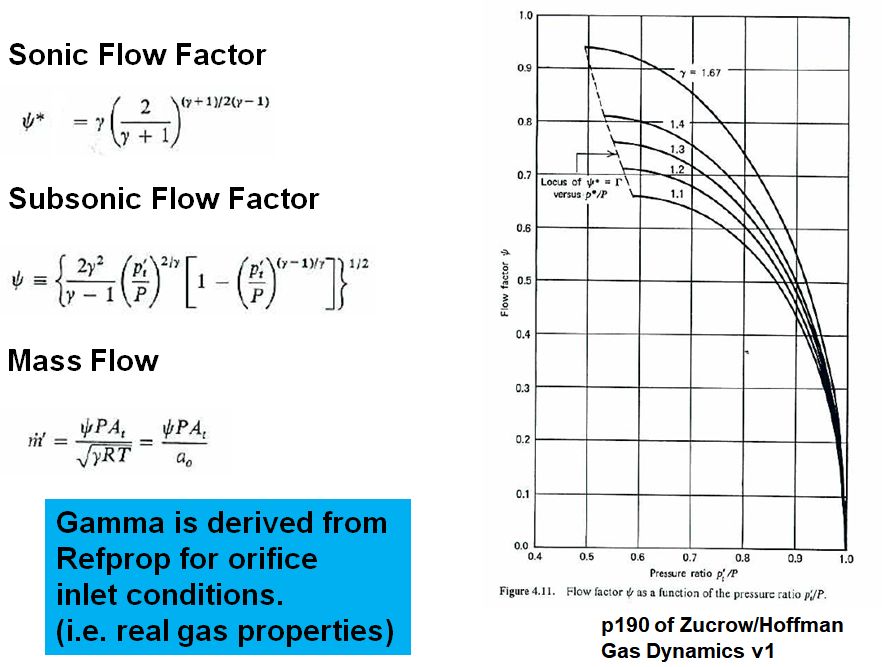
An example script to calculate a gas orifice size is:
from prism import Gas_Orifice

orf = Gas_Orifice(name="gas orifice", gasSymbol='O2',  matlName="Ti",
        CdAInp=0.1, wdot=1.1, TgasDegR=530.0,
        usePinlet=0, PgasOutlet=400.0, PgasInlet=400.0,
        Number=1, sf=4.0, cxw=1.25)

print orf.getSummary()
and give the following output:
Gives Output:
Gas Orifice: gas orifice
             mass =        0.003 lbm
             type = inert
        In: O2 T= 530.0 P= 521.3 D=3.0013 E= 79.18 H=111.34 S=1.301 Supercrit
        Out:O2 T= 526.1 P= 400.0 D=2.3098 E= 79.28 H=111.34 S=1.317 Supercrit
        fluid : O2
        Structural Material : Ti
        Allow Non-Standard wall thickness
        Using Poutlet to design Orifice
        Orifice CdA is an Input
        Orifice is SUB-SONIC
     ==== INPUT ====
        wdot            = 1.1 lbm/sec
        SCFM            = 797.491 SCFM
        CdAInp          = 0.1 in
        PgasOutlet      = 400.0 psia
        sf              = 4
        cxw             = 1.25
        # Orifices      = 1
     ==== OUTPUT ====
        PgasInlet       = 521.3 psia
        velFPS          = 527.77 ft/sec
        dpOrifice       = 121.32 psid
        dp/Pinlet       = 0.232717
        thkWall         = 0.030 in
        rinsid          = 0.178 in
        dinsid          = 0.357 in
        rho             = 0.16 lbm/cuin
        sy              = 119000 psi
        tming           = 0.030 in
        fluid dens      = 3.00131 lbm/cuft
        fluid visc      = 1.41988e-05 lb/ft-sec
        fluid sonicV    = 1075.42 ft/sec
        fluid Mach      = 0.490757
Size a Gas Regulator
Similar methods as above are used to size a gas regulator:
from prism import Gas_Regulator

reg = Gas_Regulator(name="gas regulator", gasSymbol='O2',  matlName="Ti",
        wdot=1.0, TgasInit=530.0, TgasFinal=400.0,
        PgasOutlet=400.0, PgasInit=4000.0,  PgasFinal=800.0,
        Number=1, CdASF=1.5, sf=4.0, cxw=1.25)

print reg.getSummary()
Gives Output:
Gas Regulator: gas regulator
             mass =        0.244 lbm
             type = inert
        Initial:
        In: O2 T= 530.0 P=4000.0 D=23.2378 E= 59.45 H= 91.32 S=1.143 Supercrit
        Out:O2 T= 440.1 P= 400.0 D=2.8238 E= 65.09 H= 91.32 S=1.276 Supercrit
        Final:
        In: O2 T= 400.0 P= 800.0 D=6.7375 E= 54.27 H= 76.26 S=1.200 Supercrit
        Out:O2 T= 377.7 P= 400.0 D=3.4004 E= 54.48 H= 76.26 S=1.239 Supercrit
        fluid : O2
        Structural Material : Ti
        Allow Non-Standard wall thickness
        Final condition is SUB-SONIC
     ==== INPUT ====
        wdot            = 1 lbm/sec
        SCFM            = 724.992 SCFM
        TgasInit        = 530.0 degR
        PgasInit        = 4000.0 psia
        TgasFinal       = 400.0 degR
        PgasFinal       = 800.0 psia
        PgasOutlet      = 400.0 psia
        CdASF           = 1.5
        sf              = 4
        cxw             = 1.25
        # Regs          = 1
     ==== OUTPUT ====
        CdAInit         = 0.0094 sqin
        CdAFinal        = 0.0421 sqin
        CdA             = 0.0631 sqin
        dpRegulator     = 400.00 psig
        dp/Pinlet       = 0.5
        rinsid          = 0.142 in
        dinsid          = 0.284 in
        rho             = 0.16 lbm/cuin
        sy              = 119000 psi
        tming           = 0.030 in
        fluid dens      = 23.2378 lbm/cuft
        fluid visc      = 2.08782e-05 lb/ft-sec
        fluid sonicV    = 1317.98 ft/sec
Helium Pressurization
The sizing of a Helium pressurization system depends on:
- Helium MEOP
- Propellant Tank Pressure
- Propellant Tank Volume
- Helium ACS Requirements
- Operating Temperature Range
- Mission Time
- Regulator Delta P Requirements
- Average Acceleration
- Tankage Mass, Surface Area, Material
- External Heat Loads
Create Summary
The following script takes these into consideration.
from prism import PressurantInteg

h = PressurantInteg(name="General Test", gas='HE',
    VpropTnk=300000.0,PGasTnkMEOP=4455.0,PpropNom=180.0,
    Nbottle=4,
    PfinGasOvPnom=0.9, heatExchangerTout=None,
    tAction=400.0,TminR=510.0,TmaxR=550.0, useDBruns=0, TbottleMatlConst=None)

print h.getSummary()
Gives Output:
Helium Pressurant: General Test
             mass =       24.742 lbm
             type = pressurant
        Integrated Heat Transfer
     ==== INPUT ====
        VpropTnk        = 300000 cuin
        PGasTnkMEOP     = 4455 psia
        PpropNom        = 180 psia
        PfinGasOvPnom   = 0.9
        tAction         = 400 sec
        TminR           = 510.0 degR
        TmaxR           = 550.0 degR
     ==== OUTPUT ====
        WGasTotal       = 24.742 lbm
        WtGasResid      = 1.667 lbm
        WGasNon-Resid   = 23.075 lbm
        Vbottle         = 16117 cuin
        wdotGas         = 0.0576869 lbm/sec
        compressInit    = 1.1403
        PbottleCold     = 4135.27 psia
        densInitBot     = 2.65275 lbm/cuft
        densFinalBot    = 0.178768 lbm/cuft
        densFinalProp   = 0.138971 lbm/cuft
        gammaIsen       = 1.63927
        gamPolyBottle   = 1.14896
        gamPolyTank     = 1.01908
        fracIsenBottle  = 0.233009
        fracIsenTank    = 0.0298427
        TfinalPropGas   = 480.0 degR
        TfinalGasBot    = 335.1 degR
        PfinalGasBot    = 162.0 psia
Show Calculation Details
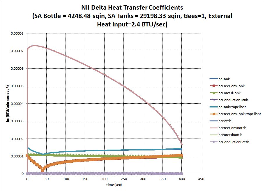
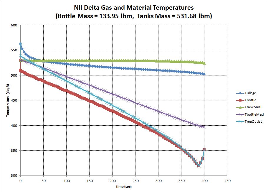
from prism import TankPress

# simulation of NII Delta He pressurization

Vfull = 5.69 * 1728.0
Voull = 5.0 * 1728.0
Vftank = 78.66 * 1728.0
Votank = 95.11 * 1728.0
Vtanks = Vftank + Votank
Vullage = Vfull + Voull
Vliq = Vtanks - Vullage
tburn = 400.0
Vbottle = 8.7 * 1728.0
Pbottle=4455.0

Peff = (Vftank*184.4 + Votank*171.0)/Vtanks

tf = TankPress(gas="HE", Vbottle=Vbottle, Vullage=Vullage, Vliq=Vliq, vdotLiq=Vliq/tburn,
    Pbottle=Pbottle, Ptank=Peff,
    Tbottle=530.0, Tullage=530.0, initTullage=1, AccGees=1.0,
    PVoW_Bottle=500000., PVoW_Tank=100000.,
    Nbottle=3, ellBottle=1.0, LcylOvDBottle=0.0, Cp_effBottle=0.125, # Cp Ti=.125, Al=.2, Monel=.1
    Ntank=2, ellTank=1.414, LcylOvDTank=1.0, Cp_effTank=0.15,
    CdARegMax=None,  NtimeSteps=100,
    QexternalIntoBottle=2.4, dPregulator=2.0 )

tf.makeExcelPlots( title='NII Delta' )
End Burning Solid Grain
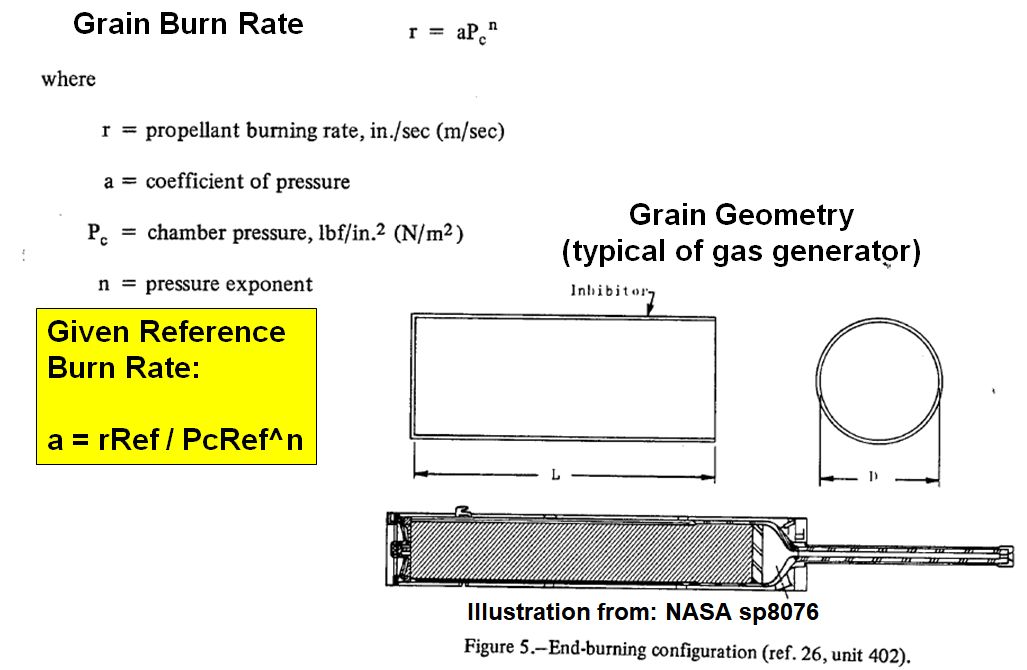
The following script.
from prism import Grain_EndBurn

grain = Grain_EndBurn(name="grain(end burner)",
        WpropBurned=200.0, propName='ARC448',
        cxw=1.0, Pc=500.0, FvacMaxPerGG=300.0, IspVacDel=238.6)

print grain.getSummary()
Gives Output:
Solid Grain (End Burning): grain(end burner)
             mass =      200.000 lbm
             type = propellant
        Propellant : ARC448
     ==== INPUT ====
        WpropBurned     = 200.000 lbm
        cxw             = 1
        FvacMaxPerGG    = 300 lbf
        Pc              = 500.0 psia
        IspVacDel       = 238.6 sec
        refBurnRate     = 0.1200 in/sec
        refPress        = 500.0 psia
        BRexp           = 0.6
        rho             = 0.0555 lbm/cuin
     ==== OUTPUT ====
        wdotMaxPerGG    = 1.25733 lbm/sec
        tminBurn        = 159.1 sec
        BurnRate at Pc  = 0.1200 in/sec
        Aburn           = 188.789 sqin
        Dgrain          = 15.504 in
        Web             = 19.088 in
        Vgrain          = 3603.604 cuin
